MEAM.Design - MEAM 247 - P2P2: Concentration - Background
Plane Stress & Strain
Given that our specimen is thin and loaded only in the plane of the plate, we will make the assumption that the stress does not vary through its thickness. This is known as a state of plane stress. As such, we need only consider two normal stress components: ($ \sigma_x $), and ($ \sigma_y $), along with one shear component, ($ \tau_{xy} $).
For an elastic element undergoing plane stress, the Poisson effect relates normal stresses to normal strains such that:
($$ \epsilon_x = \frac{1}{E}\left(\sigma_x - \nu \; \sigma_y \right) $$)
($$ \epsilon_y = \frac{1}{E}\left(\sigma_y - \nu \; \sigma_x \right) $$)
where ($\nu$) is known as Poisson's ratio and ($E$) is the Young's modulus for the particular material.
Rearranging to find ($\sigma_x$) and ($\sigma_y$), we have:
($$ \sigma_x = \frac{E}{1-\nu^2}\left(\epsilon_x + \nu \epsilon_y \right) $$)
($$ \sigma_y = \frac{E}{1-\nu^2}\left(\epsilon_y + \nu \epsilon_x \right) $$)
Net-Section Stress
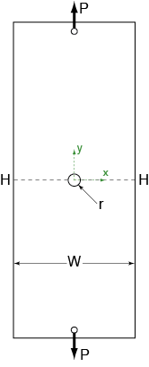
For a given cross-section through our specimen, we can define the net-section stress as the applied load divided by the load-carrying area at that cross section. Looking at the section through the midplane of our plate (the line H-H which is bisecting the hole), the net-section stress would be
($$ \bar\sigma^* = \frac{P}{(W-2r)t} $$)
Where ($P$) is the applied load, ($W$) is the width of the plate, ($r$) is the radius of the hole, and ($t$) is the thickness of the plate.
Note that this is the average stress at a given cross section. It says nothing about the distribution of stress within the section.
Stress Concentrations for Round Holes
The full analytical solution for the state of stress caused by a hole in a plate is actually rather complicated (see Timoshenko and Goodier's Theory of Elasticity, pp 90-92 for more details). To simplify matters, we will be focusing our attention to the plane bisecting the plate (H-H in the diagram above). This plane is of interest as it contains the maximum stress experienced by the entire plate, and provided that the width of the plate is much larger than the radius of the hole, there exists an exact solution for the x and y components of the planar stress:
($$ \sigma_x = \frac{3\bar\sigma^*}{2}\left(\left( r/x \right)^2 - \left( r/x \right)^4 \right) $$)
($$ \sigma_y = \frac{\bar\sigma^*}{2}\left( 2 + \left( r/x \right)^2 + 3 \left( r/x \right)^4 \right) $$)
Where ($\bar\sigma^*$) is the net section stress, ($r$) is the hole radius, and ($r<x<W/2$) is the distance from the center of the hole.
In many applications we find ourselves concerned only with the maximum stress that will be induced in an object, rather than understanding the full distribution. For this we make use of the stress concentration factor, which is a scalar value representing the increase in stress due to geometric irregularity. It is defined as the maximum value of ($\sigma_y$) divided by the net-section stress, ($\bar\sigma^*$). For the hole in the plate, the maximum stress is found when ($x=r$), which results in a stress concentration factor of 3.
In addition, we can examine the variation in stress around the circumference of the hole, which takes the form of
($$ \sigma_{\theta \theta} = \bar\sigma \left( 1 - 2\cos (2\theta)\right) $$)
where ($\bar\sigma$) is the far-field applied stress (the stress through the regular cross-section of the plate), and ($\theta$) is the angle with respect to the applied stress axis (the y axis in our case).

Point Loads and St. Venant's Principle
When a point load is applied in the plane of a plate, the stress around the load point will be non-uniform. The mathematical analysis of this problem is relatively complicated, so we shall borrow some results from literature and utilize finite-element methods (explained below) to gain some understanding of the state of stress around the point load.
The figure to the right shows a representation of the y-axis stress in a plate with a point load directed along the y-axis, centered at the top of the plate. Green corresponds to the minimum stress, while red represents the maximum stress. Regions of equal color have approximately the same stress. Examination of this figure shows that the normal stress in a section close to the point load is distinctly non-uniform, and that the further we move from the point load, the more uniform the stress becomes (which is in keeping with Saint Venant's principle). By the time we are a width's length away from the point load, we can safely assume that the stress across the section is uniform.
Photoelasticity

Every point in a loaded material experiences a state of stress. To visualize such internal stresses, we will use the fact that when certain isotropic materials are deformed, they lose isotropy in one direction, resulting in birefringence (otherwise known as double refraction). Any areas where the sample has been deformed away from the isotropic state will exhibit two different refractive indices (how much the speed of light decreases in the material) based upon the state of stress. The difference in the refractive indices results in a relative phase retardation between the two waves, causing optical interference patterns which can be observed by viewing the sample through polarizing filters. The severity of phase retardation is dependent upon the magnitudes of the principal stresses in the sample, and can be found using the Stress-Optic Law for a planar sample as:
($$ R = C t \left(\sigma_{11} - \sigma_{22}\right) $$)
where ($R$) is the magnitude of retardation in radians, ($C$) is the stress-optic coefficient of the material (units of m/N), ($t$) is the sample thickness, and ($\sigma_{11}$) and ($\sigma_{22}$) are the first and second principal stresses. From Mohr�s circle, we can recognize that the maximum in-plane shear stress is given by
($$ \tau_{max} = \frac{\sigma_{11} - \sigma_{22}}{2} $$)
and we can rearrange the Stress-Optic relationship to solve for the maximum in-plane shear stress
($$ \tau_{max} = \frac{R}{2 C t} = K N $$)
where ($K$) is the material-dependent fringe constant and ($N$) is the fringe number. For a ductile specimen in bending or axial loading, one can show that the maximum in-plane shear stress provides a reasonably good prediction of where plastic deformation (and hence failure) will initially occur. Viewed as a contour map, the interference fringe patterns correspond to points in the plane where the maximum in-plane shear stress (radius of Mohr�s circle) is constant.
Note - the interference fringes actually represent both isoclinics (loci of constant principle stress direction) and isochromatics (loci of constant maximum in-plane shear stress). When the polarizing filter is rotated, the isochromatic fringes remain constant, while the isoclinics follow the orientation of the filter.